Execution Flow
As explained in the Manual, SplitNeuron have some differences in how the neural net is conceived and set up. So, putting out data structure and execution flow is the better way to see where these differences are.
At the moment SplitUserIF.c is the only (quite) completely working example. It uses SplitNeuron.h, SplitNeuron.c and other scripts (in downloads) to simulate a self-feeding network of Integrate and Fire model units.

The way used to expose splitted neuron information is clearly shown at the beginning of SplitUserIF. The structures declared in SplitNeuron.h and implemented in SplitNeuron.c are used as globals to fulfil requirements for speed and space optimization (collected in Principles) and the only flexibility for their number is given by #define: #define NUM_NEU 10000 #define MAX_CON 50 #define NUM_NEU_X 100 #define NUM_NEU_Y 100 #define NUM_ACT 1000 #define TIME 400

TARGASOMA somas[NUM_NEU]; TARGASSUM synSum[NUM_NEU]; TARGACONN phys_conn[NUM_NEU][MAX_CON]; TARGACONN *p_conn[NUM_NEU]; SReceptiveField map[2]; SCarriage carriageOut; short offsets[NUM_ACT]; Sppm imgIn, raster; char img[TIME][NUM_NEU]; char *imgOut[TIME];

Then settings for constant values and weights are read from file TestIF.set using  ReadSettings_IF()  that simply reads the file searching for particular entries and assign value to the variables used to initialize the layer.
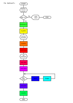
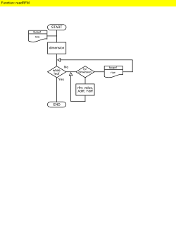
After, we use  readRFM()  function to read the receptive field map files needed to set up connections among units in the same or different layer.
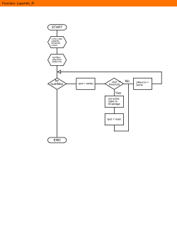
At this moment we are able to initialize completely our layer using  LayerInit_IF() . Inside this function the global structures and arrays are associated to the layer by assigning their base address to layer member variables. In addition, a random initial value (between 0 and 999+fixed amount, for IF model stays inside these limits) is assigned to each unit and, at the same time, all over-threshold units are placed inside the first SCarriage.
The connection are then assigned using  CreateConnection() . This is the longer and slower function in the project, since it is devoted to establish connection starting from one emitting layer and reaching one receiving layer (they could be even the same in case of self-exciting connections as in this exemple). As this is a more computationally treatment part, please see manual part for a general intro to these themes. The task is accomplished using layer(s) dimensions, receptive field maps and some connection schemas (only one at the moment, the others are still ToDo).
Going deeper inside this function you can see that is three-fold based on the ratio of receiver and sender:

ratio = numReceiver / numSender;

Ratio is used to separate behaviours of connection settings. If ratio < 1 there are more receiver units than sender sites, so numUnitForSite units should point to the same site as center of their receptive field map (rfm). If else ratio > 1 then there are less receiver units than sender sites and the user could choose the type of site distribution onto units. Finally if ratio == 1 receiving units and sender sites are equal: every receiver unit has its rfm center on the corresponding site and the treatment could be omological or eterological. Eterological (receiver and sender are different layer) treatment is as previous ones, omological (receiver and sender is the same layer) treatment implies joint rfm's check: neurons around are connected to the current one by superposition of receptive fields, if two neurons have receptive fields monitoring the same area, then they are connected.
In this function I took some reflection from Zhaoping Li research onto visual primary cortex, simplifing calculation to fit text-mapped spatial relations. The main idea is biologically well proofed: cells receiving same bottom-up stimuli are linked. The more their receptive fields overlap, the stronger they are connected. Using this approach, contour integration is tightly linked to orientation selectivity in a simple and effective way as it relays onto spatial-driven relations, without particularly devoted units or areas. This assumption is expressed in rfm files and the way connection function uses them. As said before, each rfm file is read and stored in SReceptiveField structures, where is represented as two-dimensional matrix of SCell structures. Every SCell keeps its value (a symbol of its polarity and nominal strenght) and its coordinate difference from the receptive field center. This latter feature has been chosen to simplify calculation during connection assignment. In addition, rfm are inteded to look at the receiving units as targets from one single emitting site, in order to ease algorithmic efficence. With little differences (pushing sooner or later to a function enclosure), receptive fields map are centered onto each emitting site, i.e. each cell linear index (as array entry) is translated into receiving layer coordinates and, starting from the map center, serves as guide to obtain a capable target on receiving layer. If a capable target is found, it is in turn converted to a receiving neuron index and appended to the layer connection array for the current emitter site.
The point is that connections are site-started. A layer owns several two-dimensional array of connections, one for each layer from which it receives activity, and all the arrays are collected into an array of pointers, since they could be different in sizes. On the inside, each array has in its first dimension the sites array, corresponding in indexes to emitter layer, so each layer has only to expose (by SCarriage) the indexes of its active units. The second dimension is the list of units covered by the site. The values stored into the matrix are TARGACONN bitfields, each containing the layer neuron index affected by the emitter active site and the twined synaptic weight.
Complexity of these data structure and functions are redeemed during execution of central loop continuously executing the main two i/o functions.
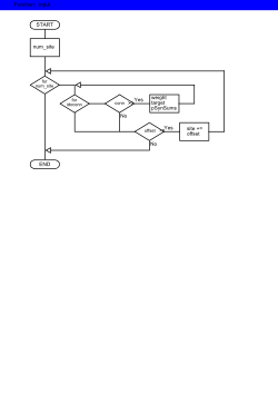
For each timestep (wishfully lasting 1ms), activity received from upstreaming layers is passed to  Input()  function, executed for each incoming SCarriage. Using TARGACONN info's, only TARGASSUM (unsigned) array entries targeted by active sites are updated, each corresponding to layer neuron synaptic sum (kept apart to ease access). Starting from the first active site index brought by SCarriage, each entry is used to access TARGACONN array. The weight stored in that connection is summed into TARGASSUM entries corresponding to every neuron connected to the active site. Then SCarriage entry is cleaned for next timestep.
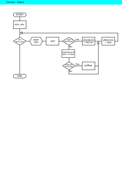
At the end of input phase all incoming stimuli have had their counterpart updated, so  Output()  function executes neuron's model activation function for each layer unit. Opposite to Input(), the output runs over every neuron in layer, taking its synaptic sum and previous instant membrane potential state and computing new state according to each model characteristic function. An hybrid solution has been set for spiking behaviour. As said here, Integrate-and-Fire model and Izhikevich´ Simple Model mainly differ in firing policy for they have different borderline zones to choose the spiking moment. I&F fires using a fake-but-simple threshold policy: whenever membrane potential trespass a certain value, the unit is said active. Simple Model uses a less simple but biologically plausible way, without a threshold: the unit fires following not strict threshold but its dynamic so algorithmic signal is peak trespassing. Depending on neuron model (choose at compile-time), the layer threspeak variable stays for one meaning and value or the other.
When the unit fires, it is added to the SCarriage active subset. An SCarriage.m_pOffset entry is filled with the current unit index, converted in offset from the previous active unit (to save representational space). At the moment an image buffer entry corresponding in index and time is also marked with ´1´, but in future release it will be subject to be treated outside, according to SCarriage (or merging them...).

Flowcharts
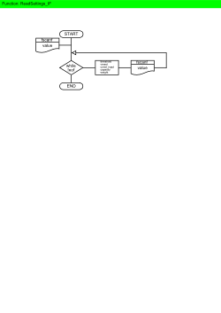
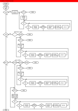
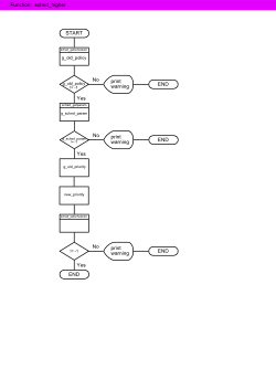
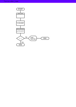
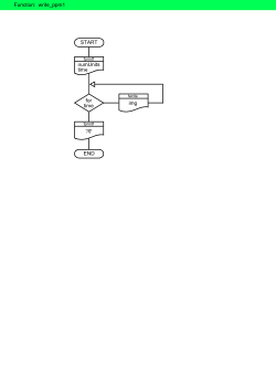
Here there are some simple flowcharts (derived from IBM Flowcharting template X20-8152) to help understanding the code and the way it is conceived.
The first flowchart is the test program "SplitUserIF.c". The colors of boxes refer to other flowcharts in the same page with corresponding header color.