

WARNING: some content is obsolete. Update under construction...
1 INTRODUCTION1.1 Unit
1.2 Architecture
1.3 Continuous vs Discrete
1.4 Network vs Population
1.5 Population activity
1.6 Applications for new models
2 MODELS
2.1 Neuron spiking
2.2 Integrate and Fire
2.3 Simple Model
3 ANALYSIS
3.1 System States
3.2 System Requirements
3.3 Develop choices
4 DESIGN
4.1 System components
4.2 Exposing and Compacting
4.3 Reorganizing execution flow
4.4 SCarriage
4.5 Connections
4.6 Receptive fields
4.7 SGroup
4.8 Memory management
4.8.1 Memory Locking
4.8.2 Scheduling
4.9 Media conversion
4.10 SLayer
SplitNeuron is a project for a set of data structures and functions being able to simulate large, biologically plausible, neural networks. This include the possibility to share load among multiple machines and calibrating operational load on each machine.
To achieve these aims, features and algorithms of usual simulation packages have been reconsidered. Most simulation tools use McCulloch-Pitts derived models which simulate neurons by a single continuous variable, representing mean firing rate. It brings well proved results so is widely used in engineering applications. But it is not biologically plausible, nor capable of reproducing activities, such as synchronization, that are needed to explain complex behaviours as recognising a pattern among others equally acceptable, keeping focus on object in a moving environment, binding shape and colour of an object, ...and many others.
These tasks are accomplished by alternative models, accurately reproducing spiking nature of neurons, i.e. the ability to rapidly change membrane potential up to the emission of a Spike. This could be interesting from an informational point of view, for the kind of computations that could be done on such signals, and from an informatics point of view, for the discreet nature of signals emitted by neurons.
The models implemented by SplitNeuron are Integrate-and-Fire (the first model showing pulsatile behaviours) and Simple Model by Izhikevich (the latest model explaining and reproducing almost all biological behaviours).
For such models there are a few simulation tools (or nothing at all) and their implementation is focused on getting knowledge ABOUT networks (statistics, dynamics, ...). SplitNeuron is concentrated on information flow INSIDE and FOR the network, aiming at the largest and fastest simulation.
1 INTRODUCTION
Due to some details in the way some terms are used throughout documentation, a brief definition is given. These are not specific explanations, so the reader is highly recommend to refer to the (many) books available on the subject for a complete explanation of basic concepts.
Top 1.1 Unit
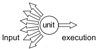
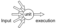
An artificial neural networks is made of a many simple units of computation interlaced called neurons, by biological inspiration. Each unit receives signals from other units trough its connections. These signals alter unit state, commonly called potential referring to membrane potential of real cells. Signals received are multiplied by a value, called weight, which simulate signal modulation of typical biological synapses. Potential value varies in time and when variation reaches a certain threshold, the unit produces a signal. Potential variation along time is a function of weighted inputs and other parameters (depending on model). Such function characterizes each model and is called ´Activation Function´ (or Transfer function, with relation to linear algebra).
Top 1.2 Architecture
The term refers to connection arrangement and units distribution. A network is made of (a lot of) units woven by connections. Units are all equal as for their functioning and differ regarding parameters and potential state. McCulloch and Pitts (1943) gave mathematical proof that a network made of such units can compute every kind of logical function due to unspecificity of unit in itself and specificity of connection arrangement and value. Indeed, every unit only treats information that is locally (to its input connection) available, without care of global purpose. Connections in and out render each unit a convergent-divergent system, the cornerstone of distributed computation. So, while architecture specifies network behaviour through signal paths, tweaking connections allows a fine tuning of activation. Therefore connections represent ´knowledge´ stored inside network and their modification can be called ´learning´. Indeed, functions modifying connections are usually called learning functions and are used to fine discriminate among data fed into networks.
Top 1.3 Continuous vs Discrete
McCulloch-Pitts Model simulates neuron activity as mean firing rate, the mean of spike fired in timeunit. In truth, neurons generate peaks of membrane potential value, known as ´Action Potentials´ or Spikes, which spread down a membrane protrusion, called axon, until they reach the end in the synapse termination, where activate (chemical) signalling to the next neuron. A spike is a short lasting event (approximately 1ms) with a stereotypical trend, therefore it is likenable to an all-or-none event (discrete, 0/1). Other mean firing rate, lots of interpretations apply to sequence of spikes (spike train) based on (arrival, relative, absolute) spike timinig. Mean firing rate works where inputs are constant or slowly changing. Only in this case, they do not require the neuron to have time reactive ability lower than that necessary to accrue postsynaptic potentials and then reach threshold. In other cases (a lot more), reactive times are shorter than those necessary to raise spiking frequency, i.e. to lower time interval between spikes. Furthermore, interpreting spike trains only as mean firing rate adds two more limitations: firstly it involves labelled lines for place of origin, because there are no other ways to identify signal origin; more, mean rate reduces to only one value the amount of information conveyed by a single channel, consequently neuron is seen as a mere integrator translating inputs sum in a single continuous value. Besides mean rate, from an informational point of view, there are other interpretations for a sequence of spikes. In general, every feature in the spike train co-varying with features of stimulus can convey information about stimulus. In addition, more codes (timing configurations) can co-exist inside the same spike frequency, so it can feed more layers of neurons able to process it differently.
On the other side, by an informatic point of view, pulse-discete nature of spikes marries operational logic of computers. This means the creation of data structures and algorithms both biological and computational suitable. Biological, as they are detailful and computational, as they are consistent with the way information is binary coded.
Top 1.4 Network vs Population
A network is defined by the model used to simulate neurons, by architecture and flow sequence. Usually a subset of units is defined ´Input units´ as they receive input values. At the same time, an ´Output units´ subset is defined to be the one to pick computed results from. This approach assumes an implicit functioning. The net starts in a ´quiet´ state (but it can be read as ´turned-off´), in which units are not active, i.e. not updated. Starting execution and applying stimuli, input units are turned-on, according to interaction among stimuli, weights and activation functions. Their activity spreads to other connected units which act just the same. At a certain moment, output units state is assumed to be the network result. This kind of functioning requires the net to have an activity state that can be treated as solution. It requires the net to go through a varying initial state to an almost fixed point state. But stability does not mean fixity. As an example, a series of values repeating in cycle can be defined as stable in time as a fixed value. New approaches in neural networks theory descend from studying them as dynamical systems and explicitly involve time in activation functions.
Furthermore, pulsed dynamical models shift stability and equilibrium concepts beyond single neuron, to the joint activity of large amount of units, or population. No wonder if some of the most important figures in neuroscience research, Walter Freeman, Gerald Edelman and Antonio Damasio, characterize neuronal ensembles on a relational/connectional/join basis. Damasio defines neuronal ensemble by connection lenght of each neuron in them; Edelman´s neuronal group is detected by join activity correlation among connected neuronal groups; Freeman brings ´gain´ key concept to distinguish aggregates, low interaction sets, from populations, high interaction ensembles showing gain during their activity in time. The main outcome of dynamic interpretation is no more existence of phases in network activity: no more input or output or converging phases, but only activity in its multiple shapes.
Top 1.5 Population activity
High connectivity degree among neurons brings subset excitations to rapidly spread through the ensemble, reaching activity level of population as a whole. This is the first feature not viewable at neuron microscopic level, spanning even over millimeters of brain cortex.
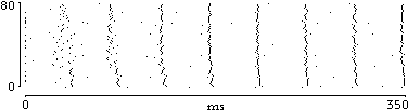 |
| fig. 1: rasterplot showing synchronization |
So, leaving single neuron, it is possible to define a ´population activity´ as the sum of active (spiking) neurons during considered time interval. Then, the more neurons are active in timeslice, the higher this population measure will be. This can be considered as a direct measure of population activity made by spike number average. In a slightly different way, taking into account an average of all membrane potentials, instant activity can be read as coherence of the population, meaning the level of activity by the number of neurons in the same state instead of the number of fired spike.
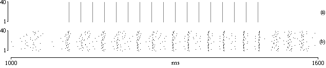 |
| fig. 2: synchronization and de-syncronization |
Synchrony and de-synchrony are claimed mechanisms to explain the way perception becomes awareness and could be projected in mind to be part of decision processes and other processes in conscience. Indeed, given a balance between absolute synchrony (epilepsy) and complete de-synchrony (noise) it is possible to figure out how a behaving (at several different level of activity) network could represent upcoming stimuli. The arrival of activity, in an already behaving network, could rapidly drive a synchronized state of a subset.
In fact, as mentioned before, this is achieved by influence of stimuli on the near-to-fire subset. Given a population with, for every timeslice, a certain number of nearly active neurons, these will be the first to be pushed to fire and start synchronization process of a bigger subset. In the same way, locally achieved coherence could be transfered to other layers where can be associated to other activations. As for local (inside a population) excitation, connections among layers cause large coherent stimuli to maximally excite large interlaced subset. At the end, as stated also by von der Malsburg, a pioneer of this kind of models, neural networks began as subsymbolic processors but can reach now symbolic processing
Top 1.6 Applications for new models
There are a lot of applications making use of spiking neuron models. Currently, major results come from perceptual problems. Categorization made with classic neural network is tied to object specific learning, along with its troubles (mainly superposition and scale limits). These can be skipped joining neural networks with expert systems explicitly treating their outputs in symbolic terms, overriding neural subsymbolic data treatment. To the contrary, spiking models, succeed in offering complete solutions to pattern analysis and storage problems:
- Binding
-
Since the same object presents itself, in natural conditions, under several variations (position, scale, rotation, perspecive deformation, illumination, background, noise, ...), there must be a way to handle this difference without ad hoc solutions. Modern neuroscience allows object features decomposition and their separate analysis as a method of variety reduction. The major drowback is subsequent binding problem: How can these spread information represent the original object as a unite whole? This task can be achieved by synchronizing populations treating different features. As a raw example, population X telling ´circle´ synchronized with population Y telling ´yellow´ are read by third population Z as ´Sun´; while population X telling ´circle´ synchronized with population Y telling ´red´ are read by third population Z as ´Mars´.
- Segmentation
-
In environments full of objects, object-ness should be a starting point in analysis. The very first stage of perception is focusing activity on one object shape (visual, auditory, ...) leaving the rest outside: the well-known figure-ground segmentation problem. This task is extremely complex for classic networks implying learning, instead is quite simple for newer model due to difference in spike train phases. Concentrating on network architecture makes possible to obtain a fine feature reacting population, fulfilling patterns and synchronizing onto them as quick as possible.
- Storage and retieval
- Learning rules of spiking models shorten times to get the network stores and retrieves fed patterns. Classic paradigms assume long learning sessions of repeated presentations and lots of examples. With spiking neurons, instead, althought hebbian algorithms are still used, learning times are greatly reduced, even to one-shot presentation and single example item.
2 MODELS
Top 2.1 Neuron spiking
To put necessary life activity through, all cells adjust in-out membrane exchanges. Lipidic membrane acts as insulator and has only channels, protein structures trespassing membrane, as control gateway. Crossing ion and molecule has chemical but also electric properties, so every body cell has a potential difference (measured in mV) between internal and external membrane side. In particular, neurons are cell fine managing their potential difference thanks to several kind of channels. Almost all of them are provided with ion chemical species selectivity and some are actually able to change their open/closed state depending on membrane potential (henceforth named voltage-dependent gates).
Cell membrane structure and behaviour can be clearly described in terms of electric circuitry (see Kandel & al[1991], appendix A). The force driving ions in and out neurons can be treated as potential difference, and ions themselves as electric charges. In the same way ion channes can be considered as conductor and cell membrane as a charge accumulator. Indeed, membrane acts as a barrier with selective permeability, carried out by channels. So it stocks non passing ion/charges. Pulled apart, charges flow into ion channels that are reasonably considered as conductors and disticted depending on their disposition to conduct charges.
To ease formalization, membrane crossing currents are split in two component: a ion current flows through channels and is treated as the conductive (ohmic) part of membrane potential (Vm) trend; while a capacitive current varies the amount of charges on both membrane sides. For a potential variation (DVm) to happen, it is necessary a variation of charges kept by membrane sides. This membrane feature gives an important property to neurons: stimuli temporal summation. Inputs coming to membrane do not vary immediatly Vm. At first the most part of charges goes to membrane wall, meeting potential difference demand, but gradually reaching (local) membrane capacity (C) limits, charges will freely flow according to electro-chemical gradient to other cell places. Finally, if input pulses, integrated in the temporal summation lapse, drive potential Vm to a certain (threshold) value, then voltage-dependent channels get activated. These channels let come in other ion species (kept until now outside) which rapidly boosts potential to voltage peak. Rapid potential change activates in turn other voltage-gated channels that let in ion species which equally rapidly lowers potential difference (hence called delay-rectifier). These events are known as spike (or action potential), which is neuron-made pulse used as signal all over the nervous system.
Lots of model have been developed simulating discrete spike emmission. This project aims two of them:
- Integrate & Fire
- Izhikevich' Simple Model
Both models use first order differential equations (or ordinary differential equations, ODE) to calculate membrane potential in time. The first one use only one equation while second uses two equations, one for rapid voltage-gated currents and the other one representing all slow delay-rectifier currents.
To implement differential equation it must be assumed a method to calculate instantaneous value increment. It can be, according to Hansel & al. [1998] sandard Euler algorithm, choosing efficency in spite of extreme accuracy.
Top 2.2 Integrate and Fire
In this model there is a big semplification: there are no voltage gated currents, as if they were completely deactivated under threshold. There are only ohmic currents (i.e. those carried by always open channels), accounting only for passive membrane properties, represented using one linear (because it uses only one differentiated variable) differential equation. In addition, if potential Vm reaches an hard threshold value, then a spike is said to fire and Vm is first automatically set to the peak value and in subsequent timeslice it is set to a low reset Vm value.
Potential dynamic under threshold is equivalent to passive membrane currents:
(1).
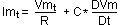
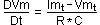
where Imt and Vmt are, respectively, membrane current and potential, R is channel resistence and C is membrane capacitance. Taking outside potential variation in time (DVm/Dt), equation (1) becomes:
(2).
To represent the spike, it is added a threshold condition for potential value:
(3). if Vmt >= threshold
when it is reached, it starts a series of prefixed assignements: first it goes to a peak value
(4). Vmt+1 = peak
and right after it is set to a very low value and kept there for a short period (tref), called ´refractary´
(5). Vmtref = reset.
This model illustrates some neuro-computational properties (as clearly pointed out by Izhikevich[2004]):
- Uniform and discrete all-or-none spike
- Defined threshold
- Refractory period
- Distinction between excitatory and inhibitory inputs, respectively pushing potential toward threshold and rest
- Input strenght encoding in spike emission frequency and temporal distiction of spike trains.
These properties make Integrate and Fire to be a model detailed enough to resemble real neuron and at the same time simple enough to grant mathematical analysis of pulsed behaviour. But, truly, it is not a real spiking neuron. That is because there not exists a fixed threshold in biological neurons, nor a completely uniform dynamic in spike upstroke. Those were semplifications made by Lapique, inventor of the model in 1907, to ease the way to formalize neuron behaviour. Indeed, spike is artificially added by conditions (3), (4) and (5), it is not a product of model equation dynamic.
Top 2.3 Simple Model
Izhikevich model is more complex from a mathematical point of view (therefore reader is highly reccomend to read his books and articles), nevertheless implemetation is quite easy, thanks to author attention to computational problems and his willingness to publish how the model has to be implemented.
Simple model, despite of name, is the most accurate from a biological point of view, without loss in computational efficency. This is the reason why has been chosen in this project. The most complete and famous model is that conceived by Hodgkin and Huxley. It consists of four non-linear (because differentiated variable are joined) differential equation accounting for membrane potential, voltage-gated and ohmic currents. Izhikevich made use of non-linear system dynamic theory to analyse and reduce quadri-dimensional Hodgkin-Huxley model to a more computational efficient bi-dimensional one. He points out how higher part of spike trend is not relevant, especially for large scale populations, compared to complex interactions among channels and currents that go under the simplified name of ´threshold´. Hence he puts in his model a differentiated variable for membrane potential and another ´recovery´ variable representing a combination of slow and voltage-gated currents. At the end, Izhikevich could leave threshold outside the model and let the model parameters and variables lead spike start. In this way he could also simulate almost all kind of neurons just changing model parameters.
Simple model is a set made of two coupled equation:
(6). DVm/Dt = Vm2 - U + I
(7). DU/Dt = a*(b*Vm - U)
where, in (6) Vm stands for membrane voltage, and in (7) U is ´recovery´ variable. Together with a and b, U renders combined interaction among ion currents. A condition similar to IF threshold is added to these equations but it represent roof-peak of spike that when reached, it is used to trigger potential reset and recovery variable update, without any mess around spike-start decision:
(8). if V >= peak
then reset potential:
(9). V = c
and update recovery:
(10). U = U + d
where parameters c and d are, respectively, reset value and instant increment. Other details on this model are too long and complex to be treated in this context, so probing readers could get complete explanations directly from author's article available on his site (see links).
Essential references:
E. R. Kandel, J. H. Schwartz, T. M. Jessell, Principles of neural science (III), Elsevier, 1991
J. A. Hertz, R. G. Palmer, A. S. Krogh, Introduction to the theory of neural computation, Addison-Wesley, 1991
W. Maass, C. M. Bishop, Pulsed neural network, Springer-Verlag, 1998
E. M. Izhikevich, "Dynamical System in Neuroscience", MIT Press, 2004
E. M. Izhikevich, "Simple Model of Spiking Neurons", IEEE Transactions on Neural Networks, 14:1569-1572
D. Hansel, G. Mato, C. Meunier, C. L. Nelter, "On Numerical Simulations of Integrate-and-Fire Neural Networks", Neural Computation, 10, pagg. 467-491
3 ANALYSIS
Models are developed to understand neural dynamics simulating it on computers. To this end, mathematical models have to be expressed in programs (computational models) in order to be executed. But natural parallel computation, that of neural biological computation, has to be brought into a single computational thread because of serial nature of common computing devices. So, balance is required between model details and computing resources (cpu speed, time access to data, memory dimensions, and so on...).
Until now, series of references have been examined to fulfil analysis and design stages of a simulation architecture capable of real-time and large number of units (complete series is here).
Top 3.1 System States
System undergoes a series of discrete states intended to simulate neural biological activities:
- Connection state change
- Activity change
- Axon state change
- Input update
- Computing activity
- Output update
The first stage is for data structure initialization and connection establishing.
The second stage is real execution in which the very three states get cyclical simulated:
- input data capture
- istantaneous unit activity
- spike encoding into output
Top 3.2 System Requirements
All the items below need to be faced during the project development:
- Large unit number
- Having a lot of units (several thousand) results in increasing the number of data structure needed to represent them. In conjunction, more of data structure means more time to compute. It is therefore necessary to search with care what are the information getting represented and how translate them into code. Due to large scaling purpose, must be planned how workload has to be treated and parcelled out among linked machines. At the same time, it is needed a way to transfer population activity simulated on a machine to others.
- Neuron models
- Project intends to support the two kinds of neuron model described before. This task is eased by common spiking dynamical nature of both model. They differ in functions and parameters but not in the way they are implemented, using standard Euler algorithm.
- Real-time
- Project core concerns data structure and functions to get neuron populations simulated. In order to make the program capable of simulating real perception tasks, it must be able to process network as fast as possible, pushing towards no delay between real and simulated reaction times. Neurons functioning mainly depends on other neurons, so in order to grant performance larger efforts will be put in representing and treating that activity.
- Different kind of inputs
- Another input neurons receive is the activity of receptors, cells specialized in encoding stimuli into spike trains. Indeed all kind of inputs cannot be fed into the network directly but need to be translated (´transduced´ in biological terms). At the same time, in every real-time application data are fed in at high speed rate. Then time needed to treat data must be shared between acquiring and translating into a network suitable form. Strategies like direct memory access (DMA) will be useful, along with devoting single machine for each external real-time data stream. That's why, as mentioned in previous points, parcel out workload has to be into project design from the beginning.
- System outputs
- Neural network outputs can be as different as the purpose for its development. The first (and sole at the moment) form of output is rasterplot. It is a graph showing lines for each neuron along time, a dot appear at point corresponding to the instant in which it fired a spike. Another very helpful could be correlation graph, showing connection activity in time. There could be other representations (visual or numeric) of instantaneous parameters state for every single neuron (membrane potential, synaptic sum, recovery variable, ...). But, to collect and keep these informations a lot of system time should be used, time that shall be used for network computation instead. The best way to achieve more outputs will be planning binary savings (such as DMA).
- User interaction
-
Users communicate with simulator by passive and active modes. User interactions should include primarily passive mode: saving data structure, states and activities. First two can be simply something like a dump, but monitor dynamic activities, for their transient nature, presents more collection problems (as stated before).
Active mode user interactions are used to vary system states in order to test perticular conditions during deployment. These kind of interactions include units and connection selective lesioning and direct input and connection changes. Both of them allow the study of system reaction. Aiming speed enhancement, the worse requirements are those of dynamic monitoring, that should be reduced to their minimum, even reduceing information supplied to the user.
Top 3.3 Develop choices
Language choice has fallen on C. Firstly because of personal familiarity with it and its diffusion. Secondly because there are a lot of online resources that brought the project (initially concived on Win platform) to develop on GNU/Linux (and eventually on Mac OSX) platform. These systems has a lot of features useful to the project:
- Lightweight: there are less task of no use during simulation (especially on graphicless interfaces)
- There are kernel modules and versions thought for real-time performance (RTAI-Linux...)
- Developer tools community granted
- System is hardware unspecific
- Platform needs no special adjustment to fit projects needs
4 DESIGN
Here are some optimization techniques to get spatial and temporal efficiency. In this section project guidelines are exposed, referring to collected hints. Some of them could be directly applied, others could be adapted to project needs and, in some cases, could not be possible to get simply the right choice but one preserving project consistence. Next exposition flanks relevant biologic features to computational features in order to explain design.
Top 4.1 System components
In this project the layer will be the main system entity, also depending on connection mode and strenght, layer will also mean population. According to neuro-computational tradition, layer is a level inside the network, made of neurons usually sharing some properties (such as connection mode or origin and cellular parameters). Some biological and computational observations would justify this choice.
First of all, neurons grow naturally in common structural and functional groups, as it is shown by pioneering work on cytologic differences by K. Brodmann.
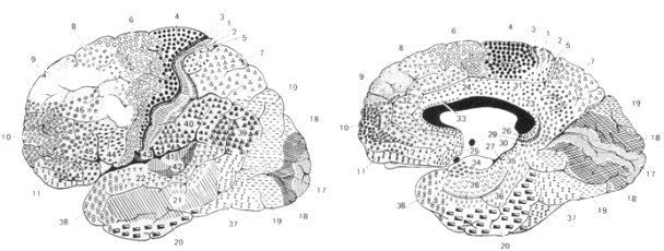 |
| fig. 3: Brodmann' maps |
As a consequence, neurons simulation shall reflect these features in parameters and applying functions. Instead of repeating the same parameters for each neuron, the layer can store general settings for its neurons with a lot of space and time efficiency.
Secondly, population activities bring more information about large network than single neurons does. Synchrony, oscillation and other events do not need specific structures for each neuron since they are derived from all population neurons.
Finally, connective relations concern population. Connection list pertain to every single neuron, but general flow directions hold between layers, indeed, seeking for afferent and efferent nerves, physiology detects lots of conections to and from an area. So, it appears that habit of enclose each dendritic tree into its neuron is correct only complying neuron cell wholeness, not connection purpose. But, obviously, there are no cells in a computer and, maybe, it is preferable trying to keep functional dynamics suggested by biology without making it more complicate.
|
Depending on the element chosen as point of view there are two usual ways to arrange network architecture: neuron oriented (better said soma oriented) or connection oriented. The former orders all informations regarding neurons (included connections) in data structure accessed by unit index. The latter does the contrary, for each connection has got a structure pointing to both neurons it affects. Keeping a neuron oriented architecture is meaningful during output to let activation function rapidly scroll through each neuron, or in case connections have to be accessed by means of owning units. But getting through units to access connections during input update slows down the process. On the contrary, connection oriented architecture is fine during input update but slows down somas accesses. The aim of this project is to make use of neither approaches, but to use them both, only where they enhance efficiency. |
To bring on this aim there shall be adopted two main strategies:
-
Splitting, exposing and making data structure compact.
It means: separating neuron data, because different informations belong to different simulation processes; easing access, declaring array of structures for each chunck of neuronal information believed capable to stand separate; keeping simple to be able to stuff more information in less data-space. Large unit number and real time need efficiency as diffuse system requirement so reducing space devoted to data and time to access them is a primary concern (see principles 7, 8, 10). -
Reorganize execution flow.
Usually choosing neuron or connection oriented architecture implies also a choice regarding how to carry out data flow, what are data to be recalled, how and when. In this case, using both approaches together, special care and special data structure are devoted to merge functional hints from biology and computational needs more than simply impose on one another.
Top 4.2 Exposing and Compacting
Since simulation runs on computer, neuron wholeness is not to be kept. Units data are split into several structure arrays, as many as functional flows require. Indipendent declaration means exposition because it removes structure-member hierarchy. Moreover, large dimension arrays will not be directly members of layer structure, there will be pointers to their base address (see principle 32).
In a develop state it is, the project could be carried on like this. But it must be able to include the best solution to manage passages of large arrays of data back and forth cache memory. This solution is blocking: knowing cache size, loops treating arrays are arranged to recall blocks of fitting size (see principles 2 and 41). That is a must since every network simulation on serial computers means keep on running along arrays.
Some principles (9, 10 and 11) point out how to get time efficiency through local treatment of variables. But the main point here is dealing with large arrays. So the solution is keep all data in global arrays (of known size at compile time and reverse storing, see principles 1 and 38) and bring up-to-needs informations into local variables with blocking principle.
That implies also compacting data. If information about one single unit is huge, only a few could be cached and treating long arrays will awkwardly imply slow disk accesses, even blocking. Indeed array dimension is determined also by the way data are stored in them. Principle 8 states it is prefereable to reduce bit fields usage, but in this case there are several information per unit to be stored, and units will be a lot. Besides, some time is spent for blocking, but it will be wasted if blocks contain only few data. So, treating large arrays, bit fields could make fast data loading because CPU cycles are less than those needed to run over large sized data. Unpack data will lose cycles but, carefully assigning manner and point of time, could be an efficient choice even for frequent use.
A further consideration in favor with compacting is accuracy needed to represent data. It depends on values extension and decimal precision. Mostly, current data types are oversized for neurons data extents. Infact membrane potential ranges between +40 mV and -80 mV, Simple Model recovery variable goes from +200 down to -200, synaptic sum has got some hundred values span. Normally double zero precision is a good balance between efficiency and accuracy. So, membrane potential (from +40.00 to -80.00) needs a variable with room for 12000 values, Simple Model recovery variable and synaptic sum (from about +200.00 to -200.00) need a variable for about 40000 values.
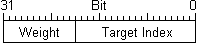
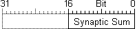
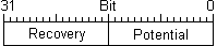
SplitNeuron has three main data type defined: TARGACONN, TARGASSUM, TARGASOMA because data used during input phase involve connections and synaptic sum, while output relevant data are synaptic sum, previous instant membrane potential and other paramenters, so they could be kept and accessed separated.
These variable are used throughout the project to declare arrays pointed by functions which access them to initialise, read and modify stored values during execution. Since bit field lenghts are declared with #define, they could be changed according to project development without compromising functions. (prefix TARGA is italian for ´plate´) |
Top 4.3 Reorganizing execution flow
In a system based on distributed analysis, structures and functions in charge of data exchange are fundamental. The core of this project points to develop a new method for encoding, transfer and decoding data regarding neurons activity. This method has to serve more layers and a lot of units in less time.
Firstly, layer is the primary system structure and units data are split into some arrays. Matter of course is unleash also activity exchange from neuron to neuron connection-twin. This could be achieved reconsidering signal transferring purpose and the way it is implemented.
Signals are sent to be computed by receivers. If a network is made of units with continuous variables, update every channel-connection each instant is meaningful, because the continuous state variable will change. But if units are spiking modelled, producing discrete outputs in time, especially at biological rate (~10 Hz), an every-instant update method will be a waste of time, because if a unit is active ten times in a second and simulated time resolution is one ms, then 9990 times that unit will be asked for no reason. Indeed, neural network simulation usually goes on like this:
 For each layer unit
- run through all of its connections
- add product of connection values for their weights to their units synaptic sum
- execute activation function with freshly changed values
Here there is an evident reversal of flow between starting position, ´each layer unit´, and its connections. Instead, previous layer activations should flow through next layer connections and then arrive to neurons owning them. SplitNeuron project, during input update, adopts connection-oriented updating system. Instead of running from a downstream unit point of view through every connection, only upstream active unit indexes are sent to next layers in the network where are used to access arrays of connection. So, the method is:
 For each active only upstream layer unit
- add product of connection values and weights to synaptic sum of only interseted neurons in next layer
- execute activation function for all next layer units
|
Property: SplitNeuron algorithm performs M*Roperations to accomplish input phase, where R=(1/A)*N , while other algorithms take M*N operation. Indeed, in SplitNeuron simulator there are M connections for N unit each, but only a ratio (1/A) of them will be active on a given timeslot. Hence for growing values of A SplitNeuron algorithm will be linearly faster than others. |
This approach implies separate and different treatment for synapses (connections) and somas (body) of units. Indeed there are already separate (exposed) arrays for connections and somas. For every layer, only active connections update is done before, and after state variables for all units are computed. This data treatment and algorithm gives the name (split-neuron) to the project. In order to realize it, a new data structure is needed, bringing upstream only active unit indexes to downstream layers and, at the same time, connection arrays have to be arranged such to be rapidly accessed from upstream side (like is done in connection oriented architecture). Next two paragraphs deal respectively with these arguments.
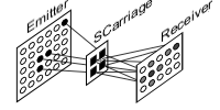
Top 4.4 SCarriage
Ensuing spike train terminology, new structure is called Carriage (SCarriage) carrying active unit indexes during trip from emitting layer to receiving ones. SCarriage does not exist in biology, it is a structure explicitly representing layer activity by means of its only active units. Activity is conceptually and practically unbound from the layer producing it. This allows a way to model biological delay between layers simply as a FIFO buffer made of SCarriages. Furthermore, the same idea could be used as a (waiting room) buffer while sending layer activities among several machines (see principles 5 and 6).
 At the beginnings, SCarriage structure contained, in one array of fixed lenght derived from layer size, just instant active unit indexes. Even though this solution was simple and temporally efficient, its space overhead was high. A fixed lenght array (say 1/10 of layer size) is a good solution but its base type should be kept as small as possible. But, in more sized layers (say thousands units), array base type would be too expensive. Indeed one byte can store indexes for a layer of only 256 units, two bytes go up to 65536 units and four bytes can take a layer of 4294967296 units. Consider that every position in this array should be as large as the last index, so the position containing low indexes will waste space.
Another solution has been proposed (Thanks to Daniele ??? and Mirko Maishberger). Array entries store not indexes directly, but offset between active units.
Now SCarriage has an int variable containing first active unit index in layer, and an array of offset containing how many units separate next active one. In any case, even this solution will need improvement, because of activity passage among machines would be carried out by some packet transfer, most probably UDP that reduces control overheads compared with TCP. But UDP packet is 8192 byte and, due to headers, available space is less. How will be stored large layer possible active unit indexes in such small space? This remains ToDo.
Top 4.5 Connections
With SCarriage, layers expose only active units. This exposition has to be prosecuted in a connection arrangement similar to connection-oriented one. These arrays are arranged in a fashion that, given the active site by SCarriage, they return the index of affected downstream units.
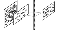
This organization follows biological evidence. Thanks to synapses among one neuron axon and other neurons dendrites, upstream layer neurons are able to modify downstream layers neurons membrane potential. In order to keep this organization consistent, downstream connection arrays have to reflect upstream layer shape, so upstream layers active sites, carried by SCarriage, trigger downstream layer connections update.
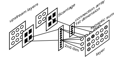 Each layer will have one bi-dimensional array for each layer it is connected to. First dimension matches the shape of emitting layer, i.e. the same number of entries as upstream layer being all possible active sites. Second dimension is a list of indexes inside downstream layer being affected by each site activity. During execution, incoming SCarriage from one of the layers connected to the current one supplies the list of active sites. This whereby, input function, following connections, updates synaptic sum of only affected downstream layer units.
Such a framework would grant a speedup during input phase, because only active connections are visited. Even if this method implies repetition on unit receiving activity from multiple upstream sites, total saving will always be more than updating every connection, especially in big sized cases.
Here can also be seen why synaptic sum is a separate array. Indeed, if synaptic sum was contained as bit field into somas array, it would slow down execution during input phase, both extracting sum field and recalling more information than necessary (which make no sense for blocking system).
Top 4.6 Receptive fields
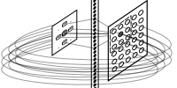
Neuron dendritic tree is usually characterized by definite spatial relations. These relations are known as receptive field and are usually represented as ´maps´ of connections distribution, strenght and polarity sign. In almost all specific litterature receptive field relations are expressed as functions, taking emitting and receiving position and other parameters, returning connection value. Procedure is certainly precise but cannot be general due to peculiarities in a lot of receptive field maps details.
Trying to ease procedure towards broader application, some assumptions have been taken. First, topological relations of receptive field need not to be tied to exact location. Second, algorithms do use current unit position, but it is a drowback of having them as functions. Indeed spatial relations are indipendent from application locus. Next step is treat receptive fields as they are represented in neuroscience manuals (see Kandel & al. [1991]), i.e. as fields or maps. The solution adopted in this project is a text file (with extension ´.rfm´, from receptive field map) containing each receptive site represented by a character and a function taking several parameters such as layer size, unit position, mean weight strenght, distribution types and so on.
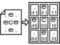 File ´.rfm´ contains a square text matrix with an odd arbitrary number of row and columns. Number has to be odd to surely have a center, corresponding to the unit which owns the receptive field. Depending on the values of the other matrix characters (named cells) connections to current unit are established. Cell values are ASCII so are quite enough for a lot of possible uses (about 224: e, i, c, +, -, ., 0, 1, 2,..., 9). Example images show the simplest file, made of only 3 cells per row and column, but it is nonetheless capable of representing different cells value (´.´ means ´no-value´; ´e´ means ´excitatory´; ´c´ means ´center´).
When rfm file is read, it is stored into a SReceptiveField structure containing an array of SCell structures. Each SCell has a character from the file and its distance from the center, expressed as coordinate difference.
Connection creation procedure follows a connection-oriented principle filtered with receptive field map because connections will be accessed from a connection-oriented point of view but downstream neuron is the field owner. Field is used to relate emitting layer units with receiving unit according to map cells values and connection function parameters.
Creating connection arrays goes on like this:
 For each emitting unit
- its index is translated into bi-dimensional coordinate
- receiver receptive field map is applied centered onto emitting unit
- all emitting units under receiver receptive field are accessed by means of map cells
- emitting units filtered are assigned to downstream connection array entries
At the end, having projected receiving unit onto emitting ones, creation procedure has been executed from emitter side with a connection-oriented mode but applying receiving neuron map and has made assignment to a connection-oriented array.
Without any change, this procedure could be used to connect the layer to itself, using a connection array that will receive in input the SCarriage output by the same layer.
In addition, map can be used directly but also be as guide applying distribution rules; used to overlay current unit map with that of a target unit pointed or nearby unit within the same layer.
Using text file representation eases complex fields creation, as an alternative to specific functions there will be specific files, so changing field is open to not initially determined cases (see principle 43). In any case, on the other side of connection method, the function is made with a switch in order to be able to add new map treatment (see principle 23).
Top 4.7 SGroup
Normally (see Kandel & al. [1991]), senses comprehend more than one receptor, coding for various submodalities (an example is somatic system, having touch, pression, temperature and pain receptors). As a consequence there are separate ways treating separete aspects of senses. These distinctions are brought up to the cortex, where it is realized a ´columnar organization´. Inside a layer, a column is a subset responding to only one kind of receptor and only for a precise localization (another example: visual cortex has got column each responding to a precise rotation of stimuli submitted to the eyes). This selectivity is obtained by a complex receptive field, a common feature of cortical neurons. A complex receptive field implies an accurate control of connections. In turn, control can be eased by subsetting units into groups, as they were a column. Structure SGroup wish to realize such demand containing pointers to layer units that are its members, so they could be easily differentiate during connective phase.
Top 4.8 Memory management
To reduce process segmentation and page faults coming from huge data segment, there are two strategies: the first one, memory locking, makes use of system function calls blocking normal paging on calling process memory pages, the second one, also using system function calls, acts on process priority to grant highest continuity of execution.
4.8.1 Memory Locking
Facing peculiar demands requires an intense use of data segment and paging mechanism is its enemy. This drowback can be prevented using system functions such as mlock() and mlockall(), which simply mark process pages so they are not swapped but kept in physical memories. In any case, growing network size, it is impossible to keep all data segment in RAM. Therefore is needed a blocking management of arrays (see principles 2 and 41). The main problem, here, is block size definition and implementation, that has to be accomplished depending on cache size, and done at compile time, before any central loop.
As an example, let tally up how much is a unit for the system:
1 unit = 4byte TARGASOMA + 4byte TARGASSUM + (4byte TARGACONN * connections)
10000 units with only 50 connections each means
TARGASOMA = ~40Kb
TARGASSUM = ~40Kb
TARGACONN = 10000 * ~200byte = ~2Mb
So, it is clear that a blocking management is needed, to organize RAM access.
4.8.2 Scheduling
Beside process memory management, CPU time management could be helpful to speed up the system. This can be done setting process priority, that manages frequency and time devoted by operating system to process access to CPU then effective execution. Reduction of processes number (see principle 5) can be easily done on a Linux system, were user can choose between graphical or not graphical interface and, more important, superuser can improve quite arbitrarily process priority (see principle 4) thanks to sched_getscheduler(), sched_getparam() and sched_setscheduler() functions.
Top 4.9 Media conversion
Project design, to be complete, should plan various kind of input media, being files or streams. Each external imput shall be transduced from its specific format into SCarriage cascade feeding layers connected to. Static simulation, making use of single files (the one implemented until now), does not need particular solution but only adequate tranlating functions. On the other hand, stream simulations, should better use DMA (direct memory access) in order to reduce CPU work to compute data.
This part, as many others are still ToDo and will benefit from any community contribution.
Top 4.10 SLayer
The structure representing each layer will then be made of pointers to:
- mono-dimensional TARGASOMA array, for all the units
- mono-dimensional TARGASSUM array, for all units synaptic sums
- one SCarriage (array) for output
- (mono-dimensional SGroup array, for connections purposes)
- total number of neurons
- constant input, membrane capacitance, reset value
- a unique variable for threshold in I&F and peak in SM (hence named threspeak)
- other variables for SM


